
Equivalent-circuit fitting turns an EIS sweep into a handful of physical parameters: solution resistance, charge-transfer resistance, double-layer capacitance, and diffusion. The fitter in Studio runs against any EIS experiment in the right sidebar.
How it works
A real electrochemical cell behaves like a small electrical
circuit. The simplest useful model is the Randles cell: a
solution resistance R_s in series with the parallel
combination of a charge-transfer resistance R_ct and a
double-layer capacitance C_dl. Each element corresponds to a
physical process at the electrode interface. R_s is the
ionic resistance of the electrolyte between working and
reference electrodes, R_ct is how hard it is for electrons to
cross the interface, and C_dl is the capacitance formed by
ions accumulating just outside the electrode.

Studio's 17 built-in circuits build on this skeleton. They add Warburg elements for diffusion, constant phase elements for non-ideal capacitance, or stacked time constants for layered or multi-step interfaces. The fitter adjusts the values of each component until the modelled impedance matches the recorded Nyquist trace as closely as possible.
Open the fitter
In the right sidebar, every EIS experiment carries a Fit badge next to its name. Click it to open the fitter for that experiment.
The badge stays highlighted while a fit is applied and greys out when no fit exists.
Pick a circuit
Studio ships with 17 built-in circuits covering most common cases: Randles, Randles with Warburg, two time constants, and their variants. Pick the one that matches the features you see on the Nyquist plot.
If none of the built-ins fit your system, switch to Custom to assemble a circuit from individual components. Drag in resistors, capacitors, CPEs, Warburgs, and connect them in series and parallel until the topology matches your system:
Building a custom circuit element by element.
Or let Studio rank all of them
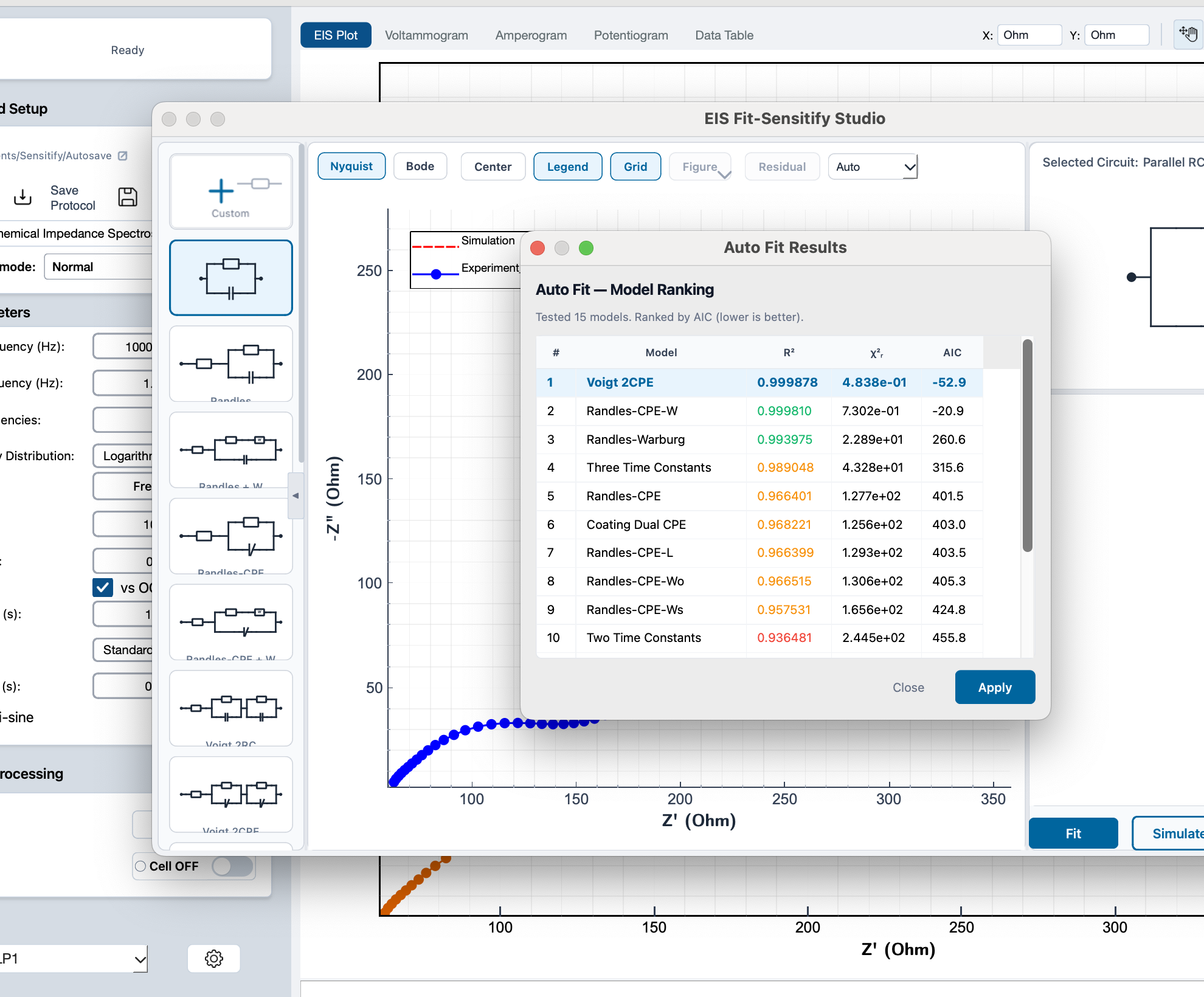
Not sure which built-in to pick? Click Auto Fit at the bottom-right of the modal. Studio runs a fit against every built-in circuit and ranks them by AIC (lower is better), showing you the best models with their R² and χ² values side by side. Pick the top entry, hit Apply, and you have your starting circuit:
Auto Fit ranks every built-in circuit and recommends the best match.
Set initial guesses
Studio auto-suggests a starting point from the data: it picks intercepts and rough magnitudes from the Nyquist trace and fills the parameter fields for you.
The auto-suggest is usually close enough for a first run. Override any value by typing into its field. This is useful when you have prior knowledge about the system or when the auto-suggest is misled by noise.
Run the fit
Press Fit in the modal. The fitter overlays the modelled impedance on the original Nyquist trace and reports the fitted parameter values with their standard errors.
The Fit badge in the right sidebar switches to its highlighted state once a fit is applied. Click the badge again later to re-open the modal and re-run with different settings.
Reading the residuals
The residuals plot shows the difference between the model and the data at every frequency. A good fit has:
- Small residuals. Below a few percent of the measured impedance.
- No structure. Residuals scattered randomly around zero, not bowing or trending across the frequency range.
Structure in the residuals usually means the circuit topology is missing a feature: a second time constant, a Warburg element, or a constant phase element where you assumed a pure capacitor.
Exclude points from the fit
A few measured points are often unreliable: high-frequency inductive artifacts from the cabling, a noisy low-frequency tail, or the odd outlier. You can leave individual points out of the fit and bring them back later, the same point-and-click way other EIS packages handle it.
The toolbar above the Nyquist and Bode plots in the fit window has two controls:
- Select points. A toggle for point-editing. It is off by default, so normal pan and zoom work until you turn it on. With it on, the cursor becomes a cross-hair and the measured points show as circle markers so you can see what is clickable.
- Reset selection. Re-includes every point.
A live read-out shows how many points are in the fit, for
example 38 / 41 points active · 3 excluded.
With Select points on:
- Click a point to drop it from the fit. It turns into a grey hollow marker; click it again to bring it back.
- Drag a box across a region, for example the noisy low-frequency tail, to exclude every point inside it.
- Cmd/Ctrl + drag a box to re-include every point in it.
Excluded points stay visible but greyed out, and they are left out of both the fit and the residuals. The measurement itself never changes. The selection is one set across all views: excluding a point on the Nyquist plot also excludes it on the Bode magnitude and phase plots, since each point is one frequency.
Changing the selection does not re-fit on its own, so dragging a box does not trigger a slow re-fit on every move. When the selection has changed since the last fit, the status shows re-fit needed; press Fit again to refit on the active points.
A few things to know:
- A fit needs at least 5 active points. Exclude more than that and pressing Fit shows a short notice instead of fitting; re-include some points and try again.
- It works alongside the frequency range from data processing: a point is used only when it is both inside that range and not excluded.
- Selection is per session. It is not saved to the file, so switching experiments or reopening the window starts fresh with every point active.
Troubleshooting convergence
If the fit fails to converge or returns unphysical values (negative resistances, capacitances many orders of magnitude off):
- Check the auto-suggested guesses. A bad starting point often sends the optimiser into a local minimum.
- Simplify the circuit. Try a simpler topology first, then add elements one at a time once each step converges.
- Drop the noisy points. Very high frequencies are often inductive and very low frequencies drifty. Exclude them with Select points above, or restrict the fit to a cleaner range in data processing.
- Repeat the measurement. Sometimes the data is just too
noisy for the model. Retake the EIS sweep with a higher mode
level (
Standard→Precision) and try again.