
Amperometry holds the working electrode at a constant potential and records the resulting current over time. It is the natural choice when the question is about a transient, a steady-state value, or the response of an electrode under a fixed bias: diffusion-limited currents, plating, sensor monitoring.
How it works
The instrument steps from the resting potential (usually OCP) to
E_DC and holds it there for the configured duration. The current
jumps to a large initial value and then decays as the analyte at
the electrode surface is consumed faster than diffusion can replace
it. Under mass-transport limitation the decay follows the Cottrell
equation, with current proportional to 1/√t. The early portion is
dominated by capacitive charging of the double layer; the late
portion approaches a small steady-state value set by diffusion.

Parameters
E_DC (V)
- What
The constant potential the electrode is held at during the run. Sets which redox process is being driven.
- Typical value
A value at which the desired process runs under mass-transport limitation: well past the half-wave potential of the analyte, but before any interfering process or solvent breakdown sets in.
- When to change
Move E_DC to switch to a different redox process, to step out of mass-transport limitation, or to probe the electrode at a specific bias for surface-state studies.
t run (s)
- What
Total duration of the step. Sets how much of the transient is captured.
- Typical value
A few seconds for fast diffusion studies or detection-limit work; tens of seconds to minutes for plating, surface-coverage measurements, or steady-state amperometry.
- When to change
Lengthen for systems that take time to reach steady state. Keep short when the early transient carries the information.
t interval (s)
- What
Time between recorded samples; the inverse of the sampling rate. Studio writes one data point per interval.
- Typical value
A few milliseconds at the start (so the fast transient is well- resolved), or a more relaxed value if you only care about the steady-state value.
- When to change
Decrease to capture fast transients faithfully. Increase to keep file sizes small for long runs where only the late behaviour matters.
Current Range
- What
Full-scale current the front-end is configured to measure. The early Cottrell transient can be much larger than the steady-state value, so the choice of range matters.
- Typical value
Pick a range that comfortably covers the expected initial peak current. The steady-state will then sit near the bottom of that range.
- When to change
Step up if the initial transient saturates. Step down if even the early peak comes in well under half full-scale. Studio flags both automatically: a live Overcurrent warning if the signal clips, and a post-run suggestion when the range is too coarse. See common issues.
Wait time (s)
- What
Pause at the resting potential before the step is applied. Lets the cell settle before the measurement starts.
- Typical value
A few seconds for stable systems. Longer when fresh electrodes need real equilibration.
- When to change
Raise it if the first portion of the trace is contaminated by an unsettled cell. Drop to 0 when the cell is already at steady state.
Demo mode (checkbox)
- What
Runs a synthesised current trace instead of measuring the cell. Useful for training, screen recordings, or testing the rest of the data path without a real instrument or sample. The Amplitude field below sets the size of the simulated signal.
- Typical value
Off for any real measurement.
- When to change
Turn on for demos and walkthroughs. Always off for analytical work.
Amplitude (V)
- What
Amplitude of the synthesised waveform produced when Demo mode is on. Greyed out and ignored when Demo mode is off.
- Typical value
0.5 V. Pick whatever makes the demo trace easy to read on the plot.
- When to change
Only matters in Demo mode. Adjust to taste.
Running it
- Connect the cell. See cell & electrode setup.
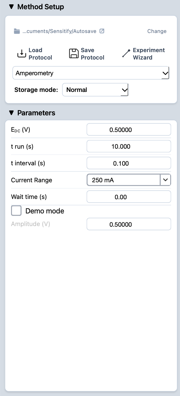
- Pick amperometry from the Method Setup dropdown and fill in the parameters.
- Press the play button at the top-left of Studio. The Amperogram tab opens automatically and the trace draws live.
- When the run finishes, the experiment appears in the right sidebar.
Reading the result
An amperometric trace typically falls from a large initial current to a smaller steady-state value as diffusion limits the current. The shape of the early transient reports on capacitive charging, the late portion on the steady-state diffusion regime.
For closer inspection of a specific region of the transient, use the marquee zoom in the plot toolbar. To compare multiple runs, leave them all visible in the right sidebar.