
Pulse voltammetry techniques apply a small potential pulse on top of a slowly stepping baseline and sample the current at specific points in each pulse. The difference between samples suppresses the capacitive background, which makes it easier to see small faradaic peaks than in a plain CV. Useful when the analyte is dilute or buried under a large charging current.
Studio offers two pulse techniques as separate entries in the Method Setup dropdown: Differential Pulse Voltammetry and Square Wave Voltammetry. Pick whichever is selected for your application.
How DPV works
DPV walks a baseline potential from E start to E end in
small E step increments and applies a short pulse at the
start of each step. Studio samples the current twice per step,
just before the pulse rises and just before it falls, then
plots the difference against the baseline potential. The
subtraction cancels most of the capacitive charging current
that dominates a plain CV, leaving a clean peak at every redox
process. The result is a peak-shaped voltammogram (resembling
the first derivative of a CV) with detection limits two to
three orders of magnitude better.

DPV parameters
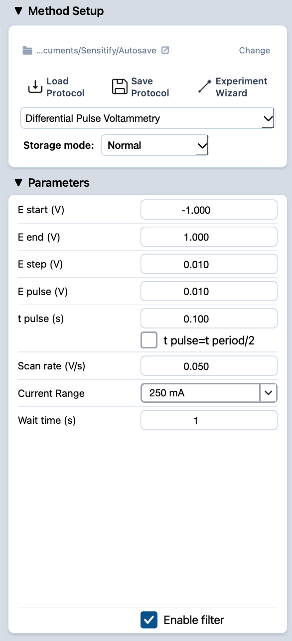
E start (V)
- What
Potential where the scan begins. Sets where the baseline staircase starts climbing from.
- Typical value
At or just below the OCP, or set 200 mV before the first expected redox peak so the baseline is clean before any faradaic process kicks in.
- When to change
Move it to skip an early process you've already characterised, or to start past a region of solvent breakdown.
E end (V)
- What
Potential where the scan stops.
- Typical value
200 mV past the last expected peak so the baseline returns to flat after the last redox process.
- When to change
Extend it when scanning unfamiliar territory; pull in to keep run times short once peaks are mapped.
E step (V)
- What
The increment by which the staircase baseline climbs between consecutive pulses. Sets the potential-axis resolution of the scan: smaller steps give a finer peak shape but more total measurements.
- Typical value
2–10 mV. Smaller for narrow peaks or close overlapping processes, larger for fast screening.
- When to change
Drop E step when peaks are sharp or overlapping. Raise it when the peak is broad and you want to finish faster.
E pulse (V)
- What
Height of the pulse applied on top of each baseline step. The size of this perturbation directly sets how strongly the faradaic process is driven during the pulse, and so how big the resulting differential current is.
- Typical value
10–50 mV. Larger amplitudes give bigger peaks (better sensitivity) but distort the peak shape and start to violate the small-perturbation assumption.
- When to change
Raise to 50 mV when SNR matters more than peak fidelity. Drop toward 10 mV for kinetic studies where the peak shape carries the information.
t pulse (s)
- What
Duration of each pulse. Shorter pulses sample closer to the moment of perturbation, capturing more of the fast faradaic response and less of the slow capacitive decay.
- Typical value
20–100 ms. Common default is 50 ms.
- When to change
Shorter pulses give higher peak currents (better sensitivity) but lose more signal to capacitive contributions. Longer pulses give lower currents with cleaner baselines.
t pulse = t period / 2 (checkbox)
- What
Locks the pulse duration to exactly half of the step period (set by
Scan rateandE step). With this on, the pulse fills the second half of every step automatically and you only adjust the timing throughScan rate.- Typical value
Off for routine work. Leaves
t pulseas a free parameter you can tune for sensitivity vs. baseline cleanliness.- When to change
Turn on when you want the duty cycle to track scan rate changes automatically (e.g. when comparing scans recorded at different rates).
Scan rate (V/s)
- What
How fast the baseline staircase climbs. Together with
E step, this sets the time between pulses (and so the total scan duration).- Typical value
1–10 mV/s. Slower than CV by design. DPV trades speed for clean baselines.
- When to change
Slow it down for the cleanest data; speed up only when throughput matters more than peak quality.
Current Range
- What
Full-scale current the front-end is configured to measure. The differential signal is small, so range selection matters more in DPV than in CV.
- Typical value
Pick the smallest range that covers the expected differential peak current without saturating.
- When to change
Drop one range if peaks come in well under half full-scale; step up if any pulse saturates. Studio flags both automatically: a live Overcurrent warning if the trace clips, and a post-run suggestion when the range is too coarse. See common issues.
Wait time (s)
- What
Pause at
E startbefore the scan begins. Lets the cell equilibrate at the starting potential.- Typical value
1–5 seconds.
- When to change
Raise it for systems that need real equilibration; drop to 0 when the cell is already settled.
How SWV works
SWV rides a symmetric square wave on top of a staircase baseline. Each step lasts one square-wave period (a forward half at the high level and a reverse half at the low level) and Studio samples the current at the end of each half. The difference between forward and reverse currents is plotted against the staircase potential. Because the square wave repeats much faster than DPV's pulse-per-step pattern, SWV finishes a sweep in a fraction of the time at comparable peak resolution.

SWV parameters
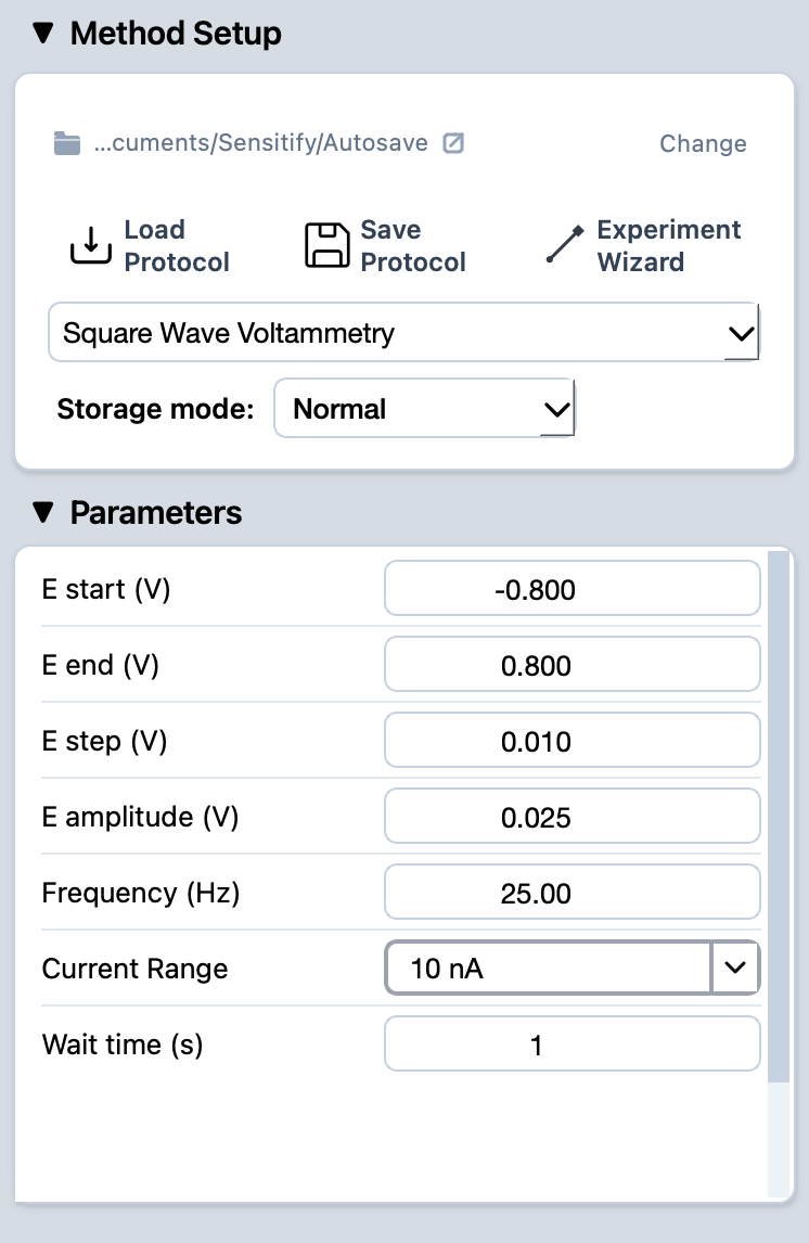
E start (V)
- What
Potential where the scan begins. Sets where the staircase baseline starts climbing from.
- Typical value
At or just below the OCP, or 200 mV before the first expected peak.
- When to change
Same as DPV. Skip an early process or start past a region you don't care about.
E end (V)
- What
Potential where the scan stops.
- Typical value
200 mV past the last expected peak.
- When to change
Extend or pull in to match the informative window.
E step (V)
- What
Increment by which the staircase climbs between consecutive square-wave cycles.
- Typical value
5–10 mV. Larger than DPV's typical step; the square wave's high frequency does more of the resolution work.
- When to change
Drop it for sharp or overlapping peaks; raise for fast screening.
E amplitude (V)
- What
Half-height of the square wave (the offset above and below each staircase level). Larger amplitudes give bigger faradaic signals but distort the peak shape and start to violate the small-perturbation assumption that keeps the analysis clean.
- Typical value
25 mV.
- When to change
Raise to 50 mV to boost peak height when SNR matters more than peak fidelity. Drop for kinetic studies where peak shape carries the information.
Frequency (Hz)
- What
Repetition rate of the square wave. Sets the time scale at which the faradaic response is probed and how fast the scan completes.
- Typical value
25–200 Hz. Higher rates emphasise fast electron-transfer kinetics and finish the scan in seconds; lower rates give cleaner peaks at the cost of total time.
- When to change
Raise the frequency for fast screening or to discriminate between fast and slow processes. Drop it for the cleanest peaks on a slow system.
Current Range
- What
Full-scale current the front-end is configured to measure.
- Typical value
Pick the smallest range that covers the expected difference-current peak without saturating.
- When to change
Drop one range if peaks come in well under half full-scale; step up if anything clips. Studio flags both automatically: a live Overcurrent warning if the trace clips, and a post-run suggestion when the range is too coarse. See common issues.
Wait time (s)
- What
Pause at
E startbefore the scan begins.- Typical value
1–5 seconds.
- When to change
Raise for slow-equilibration systems; drop to 0 when the cell is already settled.
Running it
- Connect the cell. See cell & electrode setup.
- Pick Differential Pulse Voltammetry or Square Wave Voltammetry from the Method Setup dropdown and fill in the parameters.
- Press the play button at the top-left of Studio. The Voltammogram tab opens automatically and the trace builds as the scan runs.
- When the run finishes, the experiment appears in the right sidebar under Voltammetry.
Reading the result
A pulse voltammogram is a current vs. potential trace with a flat baseline interrupted by faradaic peaks. The peak position identifies the redox process; the peak height scales with analyte concentration.
For peak picking and quantification on the trace, see find peaks and integrate a peak.