
Cyclic voltammetry is one of the most widely used techniques in electrochemistry: fast, visual, and informative about both kinetics and thermodynamics. It is the default starting point for most electrochemical work.
How it works
The instrument sweeps the working-electrode potential linearly
between two vertices, up to E vertex upper, down to
E vertex lower, and back, while recording the current that
flows in response. The forward sweep drives one half of a
redox couple, the reverse sweep drives the other. Peak
positions report on thermodynamics (the formal potential
E°'), peak separation on electron-transfer kinetics, and peak
height on both the amount of electroactive species and the
scan rate.
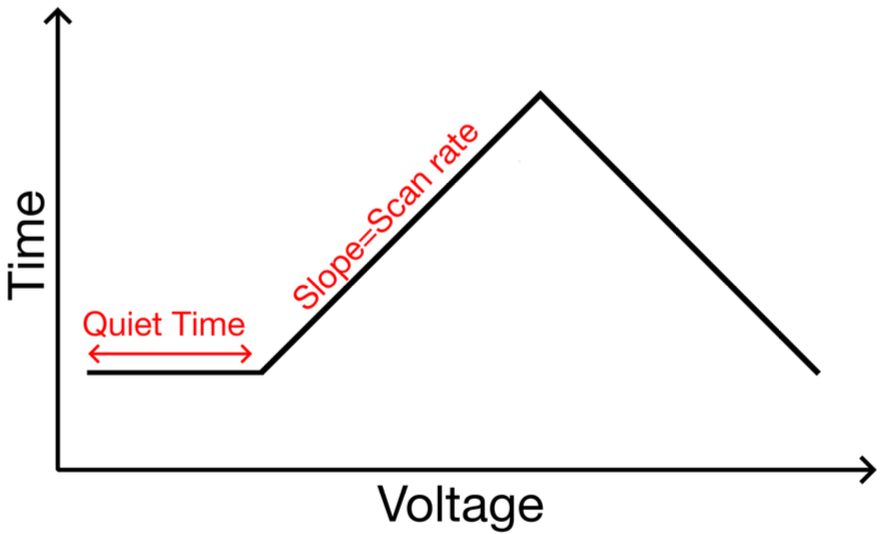
One full cycle is one triangle: the potential ramps from E start up
to E vertex upper, back down to E vertex lower, and returns. Time
runs along the X axis.
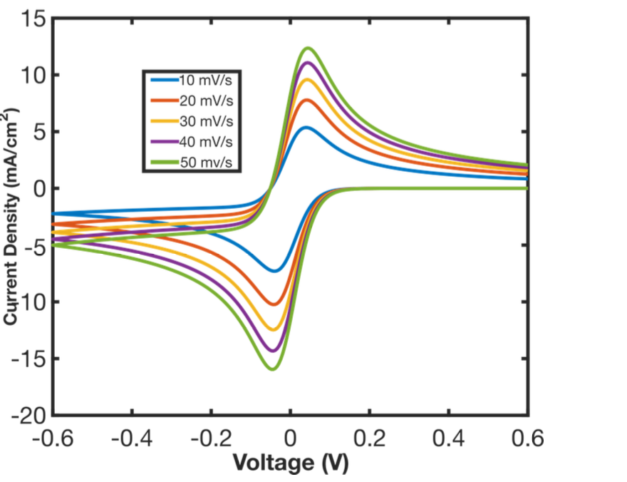
The recorded current plotted against the same potential axis. The forward sweep traces one branch of the loop, the reverse sweep the other. Peak positions report the formal potential, peak separation reports electron-transfer kinetics, peak height reports the amount of electroactive species.
Parameters
Open Studio, choose Cyclic Voltammetry from the technique dropdown, and fill in the Parameters panel.
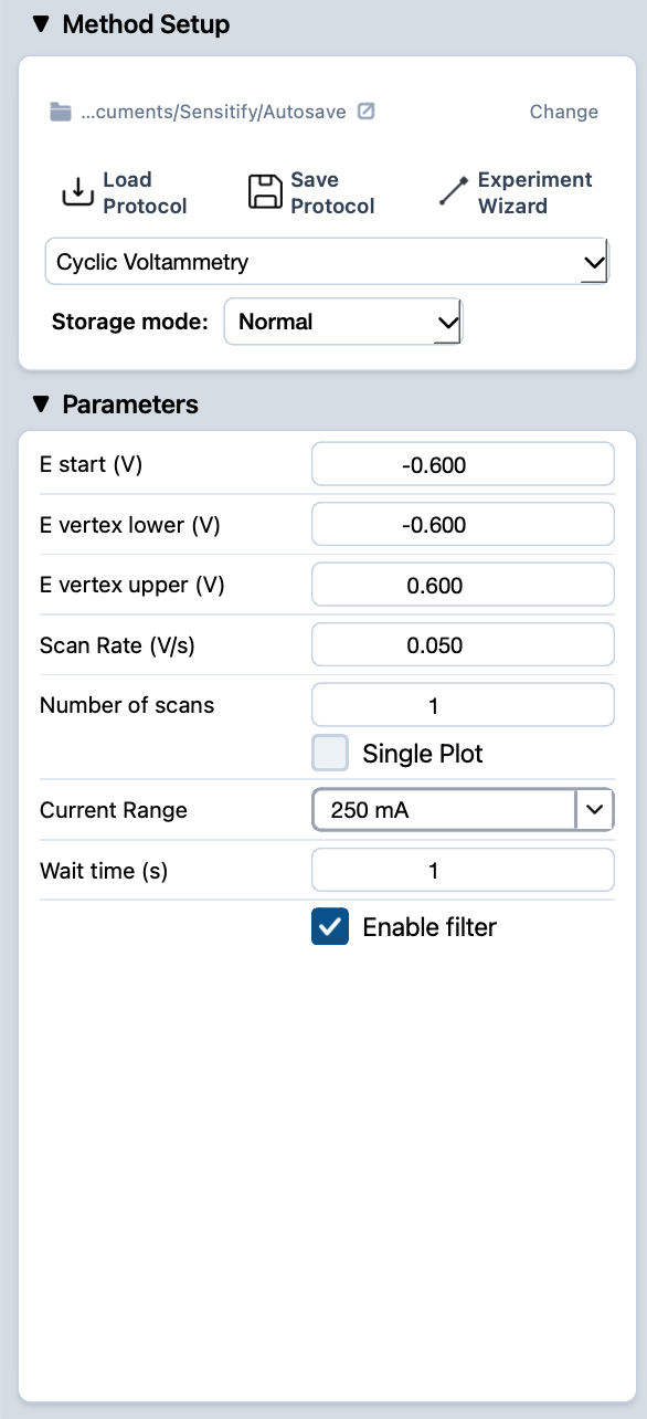
E start (V)
- What
The potential the cell is held at during the wait time, and the value the sweep ramps from when it starts. Sets where on the i-E axis the trace begins and which side of the redox process the cell sits on before any sweeping happens.
- Typical value
At or just below the open-circuit potential so the run starts in a region where no faradaic current is flowing. For aqueous redox couples this often lands somewhere between −0.5 V and +0.5 V vs Ag/AgCl.
- When to change
Move E start above OCP to begin with the analyte already oxidised, or below OCP for the opposite. Also useful for skipping an early redox process you have already characterised.
E vertex lower (V)
- What
The lower turning point. The sweep reverses direction here on its way back up.
- Typical value
Set 100–200 mV past the expected cathodic peak so the current returns to baseline before reversing. The solvent's reduction limit (hydrogen evolution in aqueous) is the practical lower bound.
- When to change
Move it more negative when scanning for new reduction processes, or pull it in to keep cycle times short once the relevant peaks are mapped.
E vertex upper (V)
- What
The upper turning point. The sweep reverses direction here.
- Typical value
Set 100–200 mV past the expected anodic peak so the current returns to baseline before the reverse sweep begins. The solvent's oxidation limit (oxygen evolution in aqueous) is the practical upper bound.
- When to change
Same logic as the lower vertex. Extend out to look for new oxidation processes, pull in once the peaks of interest are characterised.
Scan Rate (V/s)
- What
How fast the potential changes with time. Sets the time domain of the experiment, which in turn controls which physical effects dominate the trace. Slow scans are dominated by mass transport and slow kinetics, fast scans by fast electron transfer and capacitive charging.
- Typical value
0.05–0.5 V/s for routine analytical work on dissolved redox couples. Surface-confined or kinetically demanding studies can call for anything from 5 mV/s to 50 V/s.
- When to change
Lower the scan rate to resolve slow kinetics or to give thermodynamically driven processes time to equilibrate. Raise it to emphasise fast electron transfer; expect peak heights to scale with √v (Randles–Ševčík), so a 4× higher scan rate gives roughly 2× the peak current.
Number of scans
- What
How many full cycles to record. Each cycle goes from E start to a vertex, to the other vertex, and back.
- Typical value
1 for analytical work where the first scan carries the information. 5–10 for surface-conditioning experiments where the electrode needs to settle into a steady state.
- When to change
Add cycles when you need to see the trace stabilise (new electrode, contamination check). Drop to 1 to keep run times short once the system is known to be steady.
Single Plot
- What
A toggle that controls how multiple cycles are drawn. When on, every cycle is concatenated into one continuous trace. When off, each cycle is overlaid as a separate line so you can compare scan-by-scan.
- Typical value
Off for analytical work where comparing cycles matters. On for long conditioning runs where only the overall progression is interesting.
- When to change
Off when scan-to-scan changes matter. On when only the final cycle (or the long-term envelope) is relevant.
Current Range
- What
The full-scale current the front-end is configured to measure. Sets both the maximum current readable without saturating and the resolution available within that range.
- Typical value
Pick the smallest range that comfortably covers the expected peak current. For aqueous redox couples on macroelectrodes this is often the 1 mA or 10 mA range. For microelectrodes or low concentrations, drop to 100 µA or below.
- When to change
Drop one range if peaks come in well under half of full-scale to gain resolution. Step up if any part of the trace clips at the rails. Studio flags both automatically: a live Overcurrent warning if the trace clips, and a post-run suggestion when the range is too coarse. See common issues.
Wait time (s)
- What
How long the cell is held at E start before the sweep begins. Lets transient currents from the initial polarisation decay before the measurement starts.
- Typical value
1–5 seconds for routine work. Longer for systems that need real equilibration (slow adsorption, surface restructuring).
- When to change
Raise it if the first half of the first cycle looks distorted by a settling transient. Drop it (or set to 0) when the experiment needs to start as soon as possible.
Running a CV
- Connect the cell. See cell & electrode setup for the pinout and fixtures.
- Set the parameters above. The defaults are a reasonable starting point for an aqueous redox couple.
- Press the play button at the top-left of Studio. The Voltammogram tab opens automatically and the trace draws live as the sweep runs.
- When the run finishes, the experiment appears in the right sidebar under Voltammetry.
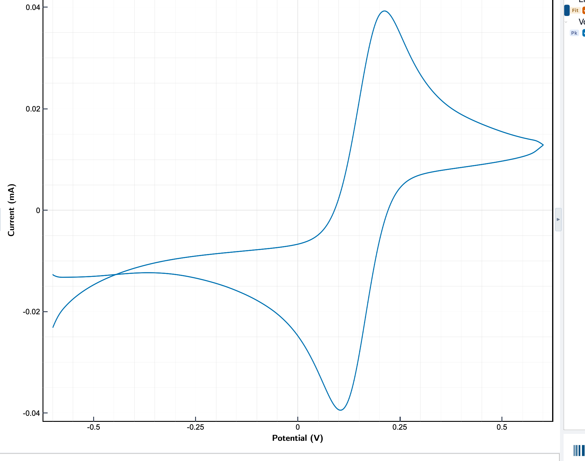
Reading the result
A clean cyclic voltammogram shows a forward sweep peak and a matching reverse sweep peak. Their separation, height, and the charge under each one tell you about kinetics, surface coverage, and reversibility.
For peak-by-peak analysis on the trace you just recorded, see find peaks and integrate a peak. To clean up the signal or restrict it to a range or cycle, see data processing.