
Electrochemical impedance spectroscopy applies a small AC perturbation across a range of frequencies and records the complex impedance at each one. It separates fast and slow processes that overlap on a CV (solution resistance, charge transfer, double-layer capacitance, diffusion) into different regions of the frequency response.
How it works
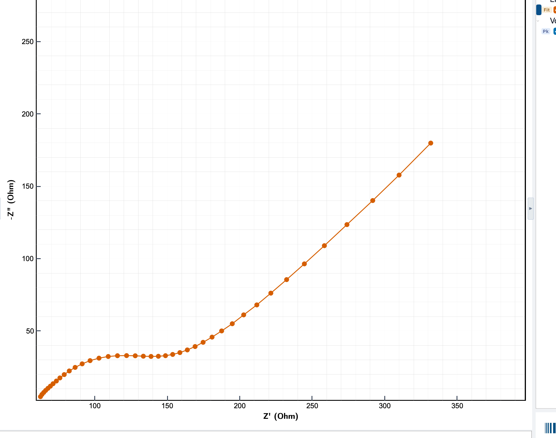
The instrument applies a small AC voltage perturbation (10 mV is a common default) on top of a steady DC bias and records the resulting AC current at each frequency in the sweep. The complex ratio of voltage to current at every frequency is the impedance Z = Z′ + iZ″; its real and imaginary parts trace out a Nyquist diagram as the frequency sweeps. Different physical processes dominate at different frequencies, so the shape of the trace separates them. Uncompensated resistance shows up at high frequencies (left of the Nyquist), charge transfer as a semicircle in the middle, and mass transport as a 45° tail at low frequencies.

Three assumptions underlie the analysis: the system has to be linear at the chosen amplitude (small perturbation), time-invariant for the duration of the sweep (steady state), and causal (the response comes from the excitation). Studio's parameter defaults are chosen to keep all three reasonable for typical electrochemical systems.
Two modes: EIS (Potentio) and gEIS (Galvano)
Studio offers two impedance modes as separate entries in the Method Setup dropdown:
- EIS (Potentio mode). Apply a small AC voltage on a DC bias, measure the resulting AC current. The default. Best when the cell sits naturally near a stable potential and the voltage is the variable you control in your experiment.
- gEIS (Galvano mode). Apply a small AC current on a DC current bias, measure the resulting AC voltage. Useful for systems where the natural variable is current: batteries during charge or discharge, fuel cells under load, electrodeposition, corrosion measurements.
Both modes follow the same parameter shape; the perturbation
and bias are expressed in volts (VAC, VDC) for EIS and in
amps (IAC, IDC) for gEIS. The frequency sweep, mode level,
and multi-sine settings are identical.
Parameters
Open Studio, choose EIS (or gEIS) from the technique dropdown, and fill in the Parameters panel.
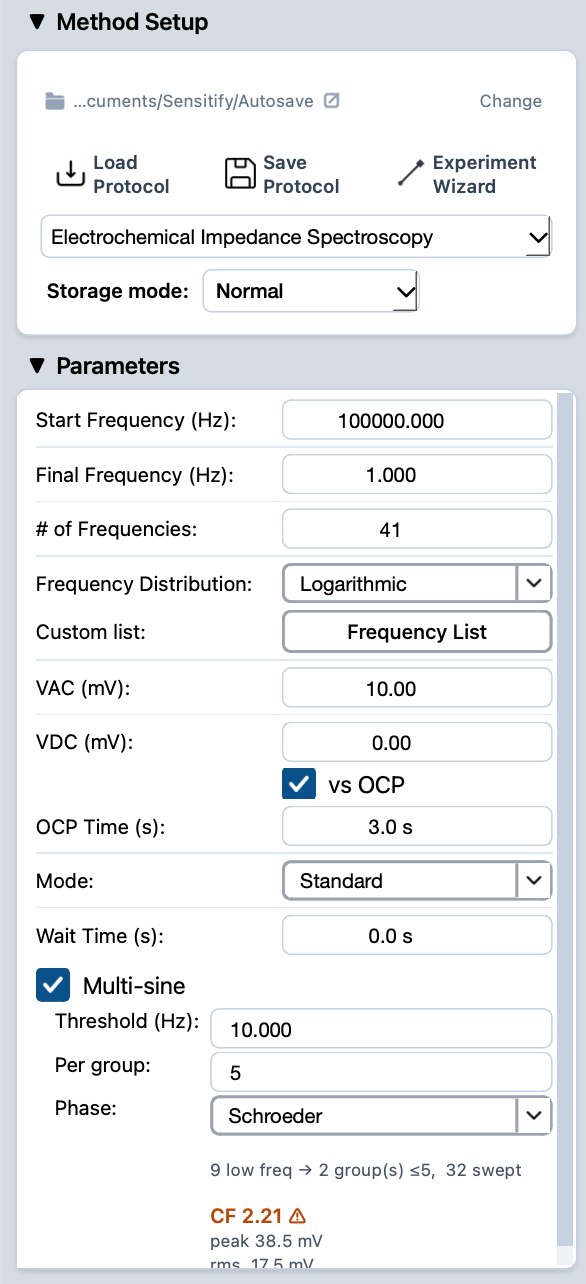
Start Frequency (Hz)
- What
The highest frequency in the sweep. Defines the short-time-scale processes the measurement can resolve. Uncompensated resistance, very fast electron transfer, and double-layer charging show up here.
- Typical value
100 kHz for routine work. Push toward 1 MHz (LP1 / 5M) when fast processes or low capacitance matter; the 5M reaches 5 MHz for thin-film and biosensor work.
- When to change
Lower it if the instrument can't reach your nominal upper bound (cable inductance, cell geometry). Raise it for systems with very fast kinetics.
Final Frequency (Hz)
- What
The lowest frequency in the sweep. Defines the long-time-scale processes. Diffusion, slow adsorption, and relaxation phenomena emerge in the low-frequency tail.
- Typical value
10 Hz to 100 mHz for routine kinetic studies. 10 mHz or lower for batteries and corrosion, where slow mass-transport effects matter.
- When to change
Lower for diffusion-dominated or battery-style measurements. Raise to keep total measurement time short when the low-frequency tail isn't informative.
# of Frequencies
- What
Total number of points across the chosen frequency range.
- Typical value
40–60 points for a routine sweep. Each extra point adds measurement time, especially at low frequencies where each cycle takes seconds.
- When to change
More points give a smoother Nyquist trace and better fit accuracy. Fewer points keep total run time short for batch screening.
Frequency Distribution
- What
How the points are spaced across the frequency range.
Logarithmicis the usual choice. It places the points so that each decade of frequency gets the same number of measurements, matching how impedance features tend to be spread across the spectrum.Linearputs the points equally in Hz.Customlets you supply an arbitrary list via the Frequency List button.- Typical value
Logarithmic. Almost every published EIS spectrum uses log spacing.- When to change
Linearfor narrow-band measurements focused on one resonance.Customwhen reproducing another study or targeting specific frequencies.
VAC (mV)
- What
Amplitude of the AC voltage perturbation. The whole EIS analysis assumes the system responds linearly to this perturbation. Too large an amplitude breaks the linearity assumption and the modelled equivalent circuit no longer maps to physical reality.
- Typical value
10 mV for most aqueous systems. 5 mV for strict kinetic work; up to 20 mV for noisy systems.
- When to change
Increase if SNR is poor and you can verify linearity (Lissajous figures, repeated sweeps at different amplitudes giving the same impedance). Decrease for small-signal systems where the inherent nonlinearity is strong.
VDC (mV)
- What
The DC bias the AC perturbation rides on. Sets the electrochemical state of the cell during the sweep. Different biases probe different surface conditions, redox states, or operating points (for batteries).
- Typical value
Often 0 mV vs OCP, so the sweep runs at the open-circuit potential and probes the equilibrium state without driving net current.
- When to change
Move VDC to a specific potential (with vs OCP off) to probe a particular redox state, an operating point on a polarization curve, or a state-of-charge on a battery.
OCP Time (s)
- What
How long Studio measures the open-circuit potential before the sweep begins. The averaged OCP is used as the reference when vs OCP is on.
- Typical value
3–10 seconds for stable systems. Longer for cells that drift on the timescale of the measurement.
- When to change
Raise it for slowly equilibrating cells (fresh electrodes, batteries warming up). Drop it when the cell is already at steady state.
Mode
- What
Trade-off between measurement time and signal-to-noise ratio.
Precisionintegrates the longest at each frequency, giving the cleanest data.Standardis the default.QuickandFastestshorten the integration so the sweep finishes sooner, at the cost of more scatter on each point. Fine for screening but harder to fit cleanly.- Typical value
Standard. Most published-quality data is fine in this mode.- When to change
Precisionfor the cleanest spectra (low concentrations, weak features).QuickorFastestwhen you're scanning many cells and need to see the gross shape only.
Wait Time (s)
- What
Pause between each frequency point. Lets the system settle to its new steady state before measurement starts.
- Typical value
0 seconds for stable systems. A few seconds when transitioning between very different frequencies seems to leave residual transients.
- When to change
Raise it if the highest-frequency points look erratic (the cell hasn't fully recovered between measurements). Drop to 0 to keep total time short.
Multi-sine (checkbox)
- What
Apply multiple frequencies simultaneously rather than stepping through them one at a time. Studio reconstructs the impedance at each frequency from the multi-frequency response, finishing the low-frequency tail much faster than a sequential sweep would.
- Typical value
Off for routine work. On for slowly-changing systems where the time saved matters more than the per-point precision.
- When to change
Turn on for batteries, cells that drift, or any system where the time-invariance assumption is hard to keep over a long sequential sweep.
The three fields below are only visible when Multi-sine is enabled.
Threshold (Hz)
- What
Frequencies below this threshold are grouped into multi-sine bursts; frequencies above it are still measured one at a time. Multi-sine pays off the most at low frequencies (where each cycle takes seconds), so the threshold lets you keep the fast end of the sweep clean and only batch the slow tail.
- Typical value
10 Hz. Anything from 1 Hz to 100 Hz is reasonable depending on how much of the sweep you want to batch.
- When to change
Raise the threshold to batch more of the sweep (saves time but gives up per-point precision). Lower it to keep most of the sweep sequential.
Per group
- What
How many frequencies are combined into a single multi-sine burst. More frequencies per group means fewer bursts (faster total measurement) but a more complex composite waveform with a higher crest factor.
- Typical value
- Studio shows a
CF(crest factor) indicator at the bottom of the panel; keep it under 3 to stay in the linear regime.
- Studio shows a
- When to change
Increase per-group count to finish faster; decrease if the crest factor warning lights up or the impedance starts looking distorted.
Phase
- What
How the simultaneous tones in a multi-sine burst are phase-aligned. Different phase patterns give different crest factors for the same set of frequencies.
- Typical value
Schroeder. The Schroeder phase is the standard low-crest- factor choice and is appropriate for almost every measurement.- When to change
Rarely. Switch to a different phase only if you're matching a specific published protocol or have a reason to prefer a different waveform shape.
Running an EIS sweep
- Connect the cell. See cell & electrode setup.
- Set the parameters above. For an unfamiliar system, start
with a wide frequency range (e.g. 100 kHz to 1 Hz),
Logarithmicdistribution, 40 points, 10 mV VAC. - Press the play button at the top-left of Studio. The EIS Plot tab opens automatically and points appear as each frequency is measured.
- When the run finishes, the experiment appears in the right sidebar under EIS.
Reading the result
The EIS plot defaults to the Nyquist view (-Z'' vs Z'). Use
the Nyquist | Bode segmented control in the plot toolbar to
switch to the Bode view (|Z| vs frequency, phase vs frequency)
when phase behaviour matters more than the impedance locus.
To extract physical parameters from the response, see fit a circuit. For comparison across multiple sweeps, leave them all visible in the right sidebar; they share the EIS plot type and overlay directly.