
Data Processing lets you clean up and focus a measured curve without changing the underlying data. It does two things in one place: it filters the signal to reduce noise, and it restricts the curve to a region of interest, a potential or time window, a single CV cycle, or, for EIS, the frequency range the fit uses.
The raw signal is always kept. Switch the filter off, change it, or come back after saving and reopening the file, and the original data is still there.
Open it
Right-click a curve in the experiment list or on its plot to get the Filter submenu:
- Off / Light / Medium / Strong. One-click presets. Pick one and the curve updates immediately. This covers the everyday case of cleaning up a noisy trace.
- Customize. Opens the Data Processing window for full control over the filter, its parameters, the range, and the spectrum view.
EIS curves show only Customize (EIS spectra are not smoothed; see the technique table below).
Presets
The presets are technique-aware: the same label does the sensible thing for each measurement type.
| Preset | Voltammetry (CV, LSV, DPV, NPV, SWV, ASV) | Time-domain (amperometry, chrono, OCP) |
|---|---|---|
| Light | Light Savitzky-Golay smoothing (~1 % window) | Gentle low-pass (cutoff ≈ ¼ Nyquist) |
| Medium | Moderate smoothing (~2.5 % window) | Medium low-pass (cutoff ≈ 1/10 Nyquist) |
| Strong | Heavy smoothing (~5 % window) | Aggressive low-pass (cutoff ≈ 1/25 Nyquist) |
The window scales with the number of points in the curve, so a preset behaves the same way on short and long scans. Change any parameter by hand in the Customize window and the preset row switches to Custom.
The Data Processing window
One window holds everything. It is non-modal: leave it open and keep working in the app, and it follows whichever curve you select.
Filters
Pick the algorithm under Filter:
- Savitzky-Golay. Polynomial smoothing that preserves peak shape and height. The best default for voltammograms. Parameters: Window (points averaged, odd) and Poly order.
- Moving average. A simple running mean. Parameter: Window.
- Median. Replaces each point with the median of its neighbours, removing isolated spikes without blurring the rest. Parameter: Window.
- FIR low-pass. Removes everything above a chosen frequency. Parameters: Cutoff (Hz) and Order (sharpness; Auto picks a sensible value). Needs a uniform sampling rate.
- Notch. Removes a single frequency to kill 50 Hz or 60 Hz mains interference. Parameter: Mains (50 or 60). Needs a uniform sampling rate.
All filters are zero-phase, so they do not shift peaks in time or potential.
Range and cycle
- Range. Min and max spin boxes in the curve's natural unit: mV for voltammetry, s for time-domain, Hz for EIS.
- Select on graph. Click it, then drag a region on the plot and the spin boxes fill in automatically.
- Cycle (CV only). Pick a single cycle or All. Cycles are detected automatically from the potential sweep.
Spectrum view
A collapsible Spectrum section at the bottom shows the data in the frequency domain, so you can see the noise and what the filter does to it:
- Raw spectrum (grey): where the noise lives, for example a clear 50 Hz spike.
- Filtered spectrum (green): what survives the filter.
- |H(f)| (dashed): the filter's frequency response.
- Cutoff line (orange, for FIR and Notch): drag it to set the cutoff visually and the Cutoff value updates with it.
The spectrum view needs a uniform sampling rate. For data without one the section is disabled, with a tooltip explaining why.
Apply and Cancel
- Apply keeps your changes and closes the window; the curve is shown filtered.
- Cancel discards the changes made this session; the curve returns to how it was when you opened the window.
- Closing with the title-bar ✕ behaves like Apply.
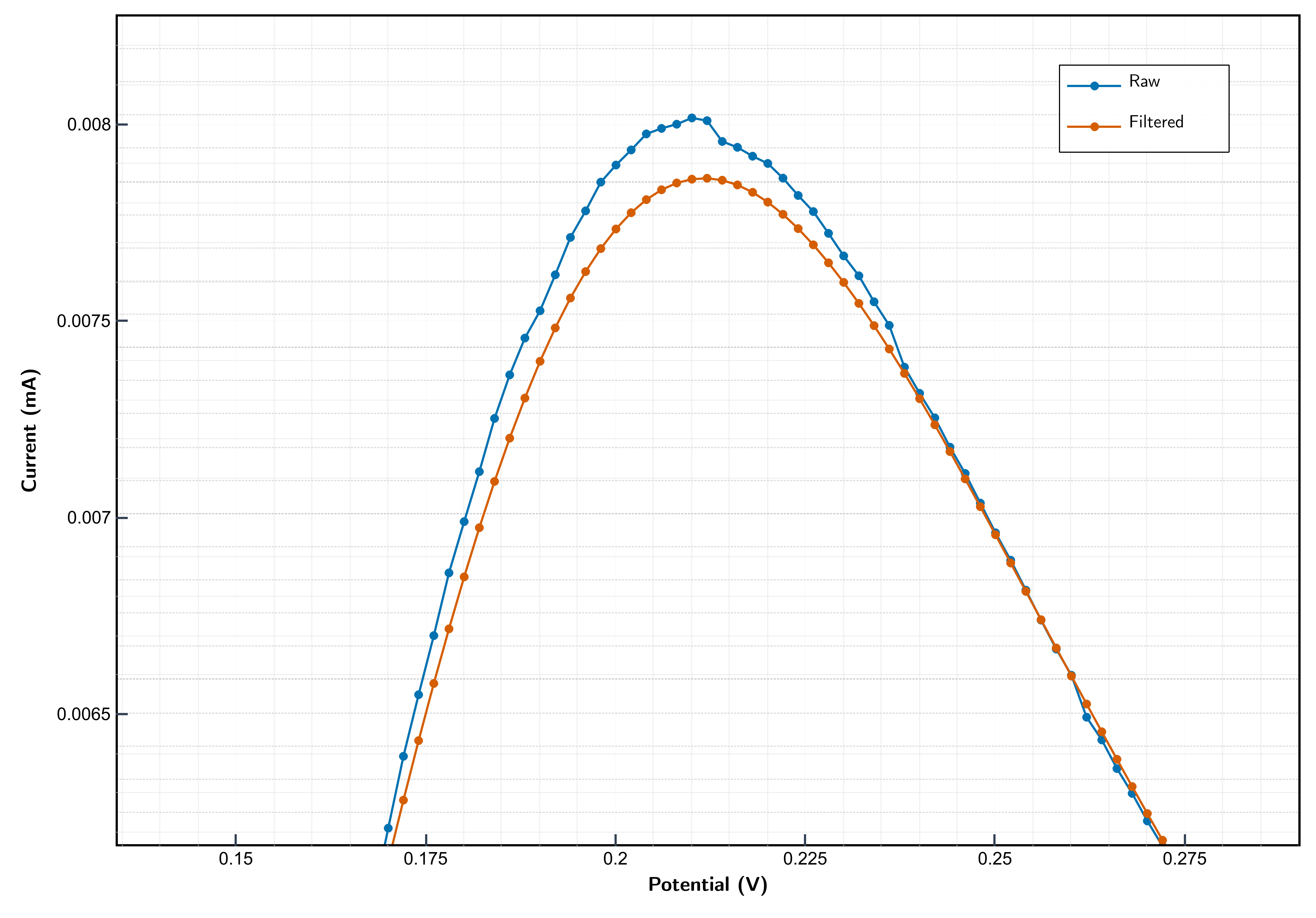
How the filtered curve appears
While the window is open, the original curve is dimmed and the filtered result is overlaid on top, so you can compare the two. Any range or cycle restriction is shown during the preview.
Once you Apply, or pick a preset from the right-click menu, the curve is shown as a single filtered trace, with no overlay and no dimming. From then on the filtered data is the curve. There is no badge or extra legend entry.
Where the filtered data goes
Once a filter is applied, the filtered series is used everywhere: the main plot (including after zoom and pan), the Data Table, and every export. Excel, CSV, ASCII, and MATLAB all write the filtered series.
The raw data is still stored in the file. Saving to .stfy records both the raw signal and the filter definition, so reopening restores the exact filtered view, and turning the filter Off brings the raw data straight back everywhere.
For EIS, the frequency range feeds the fit: with a range set, the circuit fit uses only the points inside it (Sim, Fit, and Auto-fit all respect it).
Technique support
| Technique | Smoothing filters | Range selection | Cycles |
|---|---|---|---|
| Voltammetry (CV, LSV, DPV, NPV, SWV, ASV) | Yes | Potential (mV) | CV only |
| Time-domain (amperometry, chrono, OCP) | Yes | Time (s) | No |
| EIS | No | Frequency (Hz), used by the fit | No |
FIR low-pass and Notch also need a uniform sampling rate. For the instrument's own measurements Studio derives this automatically from the acquisition settings. If a rate cannot be determined, for example in some imported files, those two filters are disabled with a tooltip, while Savitzky-Golay, moving average, and median stay available.
During a live measurement, the Data Processing controls are disabled for the recording curve and re-enable when the run stops.